Abstract | Introduction | Resource Loading | S-curves | What can be Learned?
Productivity Improvement | Learning vs. Experience | Original Theory | Two Approaches
Illustration | Issues | Conclusions | References | Appendix 1 | Appendix 2 

Appendix 2

Learning Curve Mathematics

Learning Curve Mathematics is based on the observation that when a particular task or sequence of work is repeated without interruption certain costs per unit tend to decrease in a predictable pattern. This is attributed to the experienced gained as the workers and their supervisors become more familiar with the work being repeated. There are, however, two approaches or mathematical models for purposes of practical application.

Model A: Log Linear - Cumulative Average (LL-CA)

This model was first stated mathematically in 1936 by T. P. Wright who observed that productivity improvement typically follows a constant ratio relationship in the form

For every doubling of units, the cumulative average time per unit is reduced by a constant ratio.

When plotted to log-log scale, the result is a straight line. Expressed more fully

The cumulative average time (or cost) for each of 'n' units up to the 'n'th unit, when plotted against the number of units on log-log paper, produces a straight line.

This is referred to as the Log Linear - Cumulative Average (LL-CA) Model.

Suppose the time for the first unit is taken as 100% and the ratio 'r' is 80%. then the average time for the first and second units is 80%. That is the second unit took 60% of the time of the first unit. By the time the fourth unit is reached, the average time taken for all four units is 64% and so on.

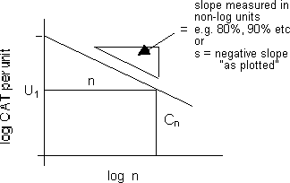
Consider Figure A1 and the following relationships.

Symbols

Figure A1: Typical learning curve plotted on a Log-Log scale

_{From Figure A1}

By definition

Model B: Log Linear - Unit (LL-U)

Model A is useful in forecasting or comparing similar operations but with significantly different numbers of units involved. It is less useful for examining results for individual units as in tracking progress on a construction site. This has led to a variation which is expressed as follows.

The time (or cost) of the 'n'th unit, when plotted against the number of units on log-log paper, produces a straight line.

This is referred to as the Log Linear - Unit (LL-U ) Model.

Again, assume that the time for the first unit is taken as 100% and the ratio 'r' is 80%. In this model, the reduction of time between the first and second unit will be 20%. Between the 2nd and 4th units it will be a further 20% and so on. That is to say, the fourth unit will take 64% of the time of the first unit. This is very different from Model A in which the fourth unit must take about 48% of the first unit.

In Figure A1 the 'y' ordinate is now 'time per unit' (rather than Cumulative Average Time per Unit). Using the symbols previously listed, the new relationship is expressed by

By definition

and

Integrating

or

and

Plotting Stage 1 of the Standard Progress Output (SPO) S-curve

In this case Model A is easier to use and the difference from Model B is minimal. By definition of the SPO S-curve, the learning curve must "force fit" to the start of Stage 2, which is one quarter of the units at one third of the time and at the slope of Stage 2 which, between points N and N+1, is two thirds.

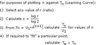
Then from equation (3) above

or

In the special case where 100% of the units are being plotted against 100% of the time, the learning curve ratio can be calculated by trial and error to 71%, or .

Thus,

or

This curve is shown plotted as Stage 1 in Figure 8. 

Appendix 1

Home | Issacons | PM Glossary | Papers & Books | Max's Musings
Guest Articles | Contact Info | Top of Page